On this page

▶

A quick ramble preamble on why I’m writing this post

TL;DR - I noticed a really cool connection between a pure math class and a CS class I was taking, and I wanted to write about it.

The vitriol I hear against maths from high schoolers frequently uses words like mechanical or dull. In higher education, that narrative seems to flip almost entirely—pure maths can be appreciated for its elegance and beauty, but it is rarely seen as a practically useful subject¹. Indeed, if forced to consider job prospects that actually use the subject material², one could be forgiven for lumping pure maths with literature and philosophy. It is the latter of these two criticisms that annoys me more. And it’s not because I don’t enjoy the beauty of mathematics (I absolutely do!). It’s because for one, I think pure maths builds an incredibly robust way of thinking³, one that rewards making progress across any point on a spectrum⁴. A conjecture is not yielding a proof? Restrict to special cases and retry. A useful tool doesn’t apply to your situation? Generalize the tool, or reframe your setup and keep trying.

But more importantly, remarkable people find ways to make ideas from pure maths useful to real-world problems all the time (and wrapping up my rant, this brings us to the actual topic of my blog post). In the spring semester of sophomore year, I took two classes straddling opposite ends of the applied-pure divide. Randomised Algorithms was motivated purely from problems in data science and Functional Analysis⁵ was, on its own, one of the most abstract classes I’ve taken. At some point in Randomised Algorithms, we studied an optimisation for a textbook matrix algorithm, and one of the pieces of that proof cited a special family of functions as a black box. Now, I really dislike rabbit-out-of-hat steps in problem-solving. And, through sheer serendipity, we studied that same family of functions in Functional Analysis that very week⁶. So, somewhat indignantly, I dove into how and why these ideas intersect, and I think the upshot of it really brings out my favourite parts of maths. That is (which my brilliantly witty title gets at), maths where the problem-solving structure follows directly from the motivating questions—form follows function⁷. Now, I’m going to share it with you.

▶A note before you continue

I direct your attention first to this rather brilliant comic. I am sure the many people working in niche research fields, who are oft asked to explain what they do to their friends and family, will relate to this.

A lot of what makes this blog post interesting is that it takes a very standard textbook algorithm and makes a clever observation about something wasteful that could be put to better use. So, I beseech you bear with me while I:

1. Convince you of the importance of the thing we’re computing in the first place,
2. Establish the textbook algorithm and its runtime,
3. Identify the wastefulness of a specific choice in that algorithm,
4. Show you how we can optimally use those wasted resources,

and perhaps then you will share my excitement in how pure maths has totally changed our intuition.

For the sake of brevity, I do assume a fair working background in linear algebra and probability. Some introductory analysis would be helpful too.

Introduction

The problem in which we are interested is computing the top-$k$ singular values and vectors of a matrix. Modern quantitative data very often comes in the form of matrices—rows and rows of data and a column for each measurable quantity. Linear algebra tells us that we can study a lot of the underlying structure of matrices through their eigenvector-eigenvalue pairs, but eigenvectors only exist for square matrices, and even then there’s no guarantee they will exist over the reals. Singular values (SVs) are the fix. Every matrix, square or not, admits a singular value decomposition $\mathbf{A}=\mathbf{U\Sigma }{\mathbf{V}}^{\top }$, where the columns of $\mathbf{V}$ (right singular vectors) form an orthonormal basis, and $\mathbf{A}$ maps that basis to an orthogonal set of directions $\mathbf{U}$ (left singular vectors), stretched by the nonnegative singular values ${\sigma }_1\ge {\sigma }_2\ge \cdots \ge {\sigma }_r>0$ sitting along the diagonal of $\mathbf{\Sigma }$.

Because we can represent any (correctly-sized) vector as a linear combination of this basis, and sitting right there in the matrix $\Sigma$ are the scaling factors we apply to each component, we realize that the dominant structural directions in our data are the singular vectors with largest singular value. More precisely, if we choose some cutoff rank $k$, then we are interested in the top $k$ singular values and vectors: $({\sigma }_1,{\mathbf{v}}_1,{\mathbf{u}}_1),\dots ,({\sigma }_k,{\mathbf{v}}_k,{\mathbf{u}}_k)$. This is the fundamental mechanism underpinning many modern data science techniques, like PCA, LoRA, KV-cache, etc.

Now, we could always compute the whole singular value decomposition (SVD), and then pick the top $k$. The textbook way to do this is to make the matrix square by computing its Gram matrix and then computing its eigendecomposition, which turns out to be enough to pick off the singular values⁸. But for problems with massive datasets⁹, this would be extraordinarily wasteful. Specifically, for $n$ rows and $d$ columns, this takes $O(n{d}^2)$ time. The first method to avoid the full SVD is an algorithm called the Power Method, which computes only the top singular value¹⁰.

---

Problem Statememt

For a matrix $\mathbf{X}\in {\mathbb{R}}^{n\times d}$, without loss of generality assume $n>d$, and let the SVD of $\mathbf{X}$ be

$$\mathbf{X}=\mathbf{U\Sigma }{\mathbf{V}}^{\top }=\sum _{i=1}^d{\sigma }_i{\mathbf{u}}_i{\mathbf{v}}_i^{\top }$$

For the matrix multiplication version (center), $\mathbf{U}\in {\mathbb{R}}^{n\times n},\mathbf{\Sigma }\in {\mathbb{R}}^{n\times d},{\mathbf{V}}^{\top }\in {\mathbb{R}}^{d\times d}$

For the outer product version (right), ${\sigma }_i\in \mathbb{R},{\mathbf{u}}_i\in {\mathbb{R}}^n,{\mathbf{v}}_i\in {\mathbb{R}}^d$ for $i\in [d]$¹¹.

We assume the usual properties of the SVD: the matrices $\mathbf{U}$ and $\mathbf{V}$ have orthonormal columns, and $\mathbf{\Sigma }$ is diagonal.

Problem: compute the top right-singular vector and value of $\mathbf{X}$ strictly faster than the SVD algorithm. That is, compute ${\sigma }_1$ and ${\mathbf{v}}_1$ in time $o(n{d}^2)$.

---

The Power Method

This outline is largely adapted from the fantastic notes from Prof. Teal Witter’s Randomized Algorithms class; all credit belongs to him.¹²

Algorithm

The first step is still to compute the Gram matrix. $\mathbf{A}={\mathbf{X}}^{\top }\mathbf{X}\in {\mathbb{R}}^{d\times d}$ which takes time $O(n{d}^2)$.

Because $\mathbf{A}$ is symmetric, it has real, non-negative eigenvalues ${\lambda }_1\ge {\lambda }_2\ge \dots \ge {\lambda }_d\ge 0$ and orthonormal eigenvectors ${\mathbf{v}}_1,{\mathbf{v}}_2,\dots ,{\mathbf{v}}_d$. Notice that the eigenvectors of $\mathbf{A}$ are exactly the right singular vectors of $\mathbf{X}$, and its eigenvalues are the squared singular values (${\lambda }_i={\sigma }_i^2$).

1. Choose ${\mathbf{z}}^{(0)}$ randomly. E.g. ${\mathbf{z}}^{(0)}\sim \mathcal{N}(0,{\mathbf{I}}_d)$.¹³
2. ${\mathbf{z}}^{(0)}={\mathbf{z}}^{(0)}/\Vert {\mathbf{z}}^{(0)}{\Vert }_2$
3. For $i=1,\dots ,m$
   1. ${\mathbf{z}}^{(i)}=\mathbf{A}{\mathbf{z}}^{(i-1)}$
   2. $n_i=\Vert {\mathbf{z}}^{(i)}{\Vert }_2$
   3. ${\mathbf{z}}^{(i)}={\mathbf{z}}^{(i)}/n_i$
4. Return ${\mathbf{z}}^{(m)}$

In short, we repeat a two-step process $m$ times: multiply our vector by $\mathbf{A}$, and then normalize it. Our final product ${\mathbf{z}}^{(m)}$ is a unit vector equal to $S{\mathbf{A}}^m{\mathbf{z}}^{(0)}$, where $S$ is just a scaling factor $S={\prod }_{i=1}^m\frac{1}{n_i}$.¹⁴

---

The important parameter $\gamma$

Now that we have it in this form with ${\lambda }_i$‘s, we must acknolwedge that our final analysis will be a guarantee based on the spectral gap parameter $\gamma$, which captures how dominant the top SV was in the dataset to begin with.

Specfically, we define

$$\gamma =\frac{{\lambda }_1-{\lambda }_2}{{\lambda }_1}$$

or more intuitively, “by what percentage must we reduce the most dominant SV, to get to the second-largest SV”.

(Intuitively, if $\gamma$ is close to $1$, the top SV is already dominant and it will be easy to isolate it. If $\gamma$ is tiny, then there’s a close battle for the top SV, so it’s tough to isolate the correct one)

---

Analysis of the Power Method

▶Full Analysis

I highly recommend reading through the full analysis to understand the machinery. However, if you choose not to, the important outcomes are the following:

• We can set our error tolerance $ϵ$ as needed, and then choose our number of iterations $m$. Our answer is guaranteed to be $ϵ$-close to the top right-singular vector
• Specifically, the minimum iterations needed is $m=O(\frac{1}{\gamma }\log \left(\frac{ϵ}{d}\right))$
• Notice that the dependence of our required iterations $m$ is only logarithmic in $ϵ$. This is very weak! We can dramatically tighten our error tolerance, and require only a modest number of extra iterations

First, by definition of $\mathbf{A}={\mathbf{X}}^{\top }\mathbf{X}$ and recalling the defined SVD of $\mathbf{X}$,

$$\begin{array}{rl}\mathbf{A}& ={\left(\mathbf{U\Sigma }{\mathbf{V}}^{\top }\right)}^{\top }\left(\mathbf{U\Sigma }{\mathbf{V}}^{\top }\right)\\ & =\left(\mathbf{V\Sigma }{\mathbf{U}}^{\top }\right)\left(\mathbf{U\Sigma }{\mathbf{V}}^{\top }\right)\\ & =\mathbf{V}{\mathbf{\Sigma }}^2{\mathbf{V}}^{\top }\\ & =\mathbf{V\Lambda }{\mathbf{V}}^{\top }\end{array}$$

where $\mathbf{\Lambda }=\text{diag}({\lambda }_1,\dots ,{\lambda }_d)$. The second equality follows from applying the transpose and noting $\mathbf{\Sigma }$ is diagonal thus symmetric; the third equality follows from orthonormal columns of $\mathbf{U}$ by definition; the fourth equality follows from $\mathbf{\Sigma }$ being diagonal and our definition of ${\lambda }_i:={\sigma }_i^2$.

So,

$$\begin{array}{rl}{\mathbf{A}}^m& ={\left(\mathbf{V\Lambda }{\mathbf{V}}^{\top }\right)}^m\\ & =\left(\mathbf{V}{\mathbf{\Lambda }}^{\mathbf{m}}{\mathbf{V}}^{\top }\right)\\ & =\sum _{i=1}^d{\lambda }_i^m{\mathbf{v}}_i{\mathbf{v}}_i^{\top }\end{array}$$

where the second equality follows from orthonormal rows of ${\mathbf{V}}^{\top }$ by definition; and the third equality from $\mathbf{\Lambda }$ being diagonal thus commuting in the outer-product version of matrix multiplication.

Recall our final answer:

$$\begin{array}{rl}{\mathbf{z}}^{(m)}=S{\mathbf{A}}^m{\mathbf{z}}^{(0)}& =S\left(\sum _{i=1}^d{\lambda }_i^m{\mathbf{v}}_i{\mathbf{v}}_i^{\top }\right){\mathbf{z}}^{(0)}\end{array}$$

We need some more useful way to represent ${\mathbf{z}}^{(0)}$. Luckily, because the eigenvectors of $\mathbf{A}$ form a complete basis of ${\mathbb{R}}^d$, we can represent ${\mathbf{z}}^{(0)}$ as a linear combination in it. Specifically,

$${\mathbf{z}}^{(0)}=c_1{\mathbf{v}}_1+c_2{\mathbf{v}}_2+\dots +c_d{\mathbf{v}}_d=\sum _{j=1}^d{c}_j{\mathbf{v}}_j$$

where the coefficients are given by the inner product $c_j={\mathbf{v}}_j^{\top }{\mathbf{z}}^{(0)}$.

So,

$$\begin{array}{rl}{\mathbf{z}}^{(m)}& =S\left(\sum _{i=1}^d{\lambda }_i^m{\mathbf{v}}_i{\mathbf{v}}_i^{\top }\right){\mathbf{z}}^{(0)}\\ & =S\left(\sum _{i=1}^d{\lambda }_i^m{\mathbf{v}}_i{\mathbf{v}}_i^{\top }\right)\left(\sum _{j=1}^d{c}_j{\mathbf{v}}_j\right)\\ & =S\cdot \sum _{i=1}^d{\lambda }_i^m{c}_i{\mathbf{v}}_i\end{array}$$

where the third equality follows from the fact that ${\mathbf{v}}_i^{\top }{\mathbf{v}}_j=\{\begin{array}{l}0\text{if}i\ne j\\ 1\text{if}i=j\end{array}$, so cross-terms in the expansion disappear.

Going back, recall that our goal is to show that our algorithm gets very close to the actual largest singular vector ${\mathbf{v}}_1$. In particular, we will show that the contribution from any singular vector that’s not ${\mathbf{v}}_1$ is arbitrarily small.

First, to separate out the error, we divide through by ${\mathbf{v}}_1$‘s coefficient, or $S{\lambda }_1^m{c}_1$. So,

$$\begin{array}{rl}\frac{1}{S{\lambda }_1^m{c}_1}{\mathbf{z}}^{(m)}& =\left(\frac{1}{S{\lambda }_1^m{c}_1}\right)\left(S\cdot \sum _{i=1}^d{\lambda }_i^m{c}_i{\mathbf{v}}_i\right)\\ & =\sum _{i=1}^d\frac{{\lambda }_i^m{c}_i}{{\lambda }_1^m{c}_1}{\mathbf{v}}_i\\ & ={\mathbf{v}}_1+\sum _{i=2}^d\frac{{\lambda }_i^m{c}_i}{{\lambda }_1^m{c}_1}{\mathbf{v}}_i\end{array}$$

where the third equality followed by simply observing that the coefficients cancel for ${\mathbf{v}}_1$ and starting the summation from $i=2$

The way we chose ${\mathbf{z}}^{(0)}$, with independent standard Gaussian coordinates, makes it rotationally invariant.¹⁵ Therefore, the distribution of $\frac{c_i}{c_1}$ for $2\le i\le d$, is $\text{Cauchy}(0,1)$, which tells us we can assume w.h.p.¹⁶ that

$$\left|\frac{c_i}{c_1}\right|\le d^3$$

Next, using our parameter $\gamma$

$${\left(\frac{{\lambda }_i}{{\lambda }_1}\right)}^m={\left(1-\frac{{\lambda }_1-{\lambda }_i}{{\lambda }_1}\right)}^m\le (1-\gamma {)}^m,$$

And we can apply the standard bound from the Taylor series of $e^x$ to claim

$$(1-\gamma {)}^m\le e^{-\gamma m}$$

Thus, if we conveniently¹⁷ choose $m=\frac{\log (d^3\sqrt{d/ϵ})}{\gamma }$, we get

$$\begin{array}{rl}(1-\gamma {)}^m& \le e^{-\gamma \cdot \frac{\log (d^3\sqrt{d/ϵ})}{\gamma }}\\ & =\frac{\sqrt{ϵ/d}}{d^3}\end{array}$$

and since we showed above that $|c_i/c_1|\le d^3$, we get that

$${\left(\frac{{\lambda }_i}{{\lambda }_1}\right)}^m\cdot \left|\frac{c_i}{c_1}\right|\le \frac{\sqrt{ϵ/d}}{d^3}\cdot d^3\le \sqrt{ϵ/d}$$

w.h.p.

Next, given that $\left|\frac{{\lambda }_i^m{c}_i}{{\lambda }_1^m{c}_1}\right|\le \sqrt{ϵ/d}$ based on our choice of $m$, we claim:

For all $i\ne 1$, either $\Vert {\mathbf{v}}_1-{\mathbf{z}}^{(m)}{\Vert }^2\le 2ϵ$ or $\Vert -{\mathbf{v}}_1-{\mathbf{z}}^{(m)}{\Vert }^2\le 2ϵ$.¹⁸

Proof.

Recall from the steps of our algorithm that ${\mathbf{z}}^{(m)}$ was normalized, i.e. a unit-vector. So, in the orthonormal basis of $\mathbf{V}$, none of its components could have magnitude greater than $1$. So, the first coefficient $S{\lambda }_1^m{c}_1\le 1$. Therefore starting from our previous result,

$$\begin{array}{rl}\left|\frac{{\lambda }_i^m{c}_i}{{\lambda }_1^m{c}_1}\right|& \le \sqrt{ϵ/d}\\ \left|\frac{S\cdot {\lambda }_i^m{c}_i}{S\cdot {\lambda }_1^m{c}_1}\right|& \le \sqrt{ϵ/d}\\ \left|S{\lambda }_1^m{c}_1\right|\cdot \left|\frac{S{\lambda }_i^m{c}_i}{S{\lambda }_1^m{c}_1}\right|& \le 1\cdot \sqrt{ϵ/d}\\ \left|S{\lambda }_i^m{c}_i\right|& \le \sqrt{ϵ/d}\end{array}$$

Again using the unit-vector property, the sum of squared coefficients must be $1$. That is,

$$(S{\lambda }_1^m{c}_1{)}^2+\sum _{i=2}^d(S{\lambda }_i^m{c}_i{)}^2=1$$

But,

$$\sum _{i=2}^d(S{\lambda }_i^m{c}_i{)}^2\le \sum _{i=2}^d(ϵ/d)\le ϵ$$

So, $(S{\lambda }_1^m{c}_1{)}^2\ge 1-ϵ$ and therefore so too is $|S{\lambda }_1^m{c}_1|\ge 1-ϵ$

For any unit vector $\mathbf{x}$, we have $\Vert \mathbf{x}-{\mathbf{z}}^{(m)}{\Vert }_2^2=2-2⟨\mathbf{x},{\mathbf{z}}^{(m)}⟩$. Since $⟨{\mathbf{v}}_1,{\mathbf{z}}^{(m)}⟩=S{\lambda }_1^m{c}_1$, we conclude that either $⟨{\mathbf{v}}_1,{\mathbf{z}}^{(m)}⟩\ge 1-ϵ$ or $⟨-{\mathbf{v}}_1,{\mathbf{z}}^{(m)}⟩\ge 1-ϵ$.

Suppose without loss of generality it’s the first: $⟨{\mathbf{v}}_1,{\mathbf{z}}^{(m)}⟩\ge 1-ϵ$. Then we would conclude that:

$$\Vert {\mathbf{v}}_1-{\mathbf{z}}^{(m)}{\Vert }_2^2=2-2⟨{\mathbf{v}}_1,{\mathbf{z}}^{(m)}⟩\le 2-2(1-ϵ)=2ϵ.$$

Thus, we conclude our proof that with only logarithmic dependence on our tolerance $ϵ$ and dimension $d$, the power method returns a good approximation for top right-singular vector.

---

As we saw above, the big influence is $\gamma$. We would be remarkably lucky if the data’s structure were represented by just one dominant vector direction, but often even highly structured data has a handful of important directions. Then, the gap from the first to second ${\lambda }_1-{\lambda }_2$ could be tiny, and $1/\gamma$ would shoot up dramatically and ruin our runtime. The Lanczos method, which we will now see, brings this dependence down dramatically to $O(\frac{1}{\sqrt{\gamma }})$.

---

The Lanczos Method

The first important observation of this method requires us to scrutinize what we actually computed during the Power Method. In particular, the most efficient way for us to get to our final product $S{\mathbf{A}}^m{\mathbf{z}}^{(0)}$ was to do $m$ matrix-vector computations, computing each ${\mathbf{A}}^i{\mathbf{z}}^{(0)}$ for $i\in [m]$

In doing so, we actually computed all the pieces of what we call a Krylov Subspace, which by definition is any subspace generated by starting with a single vector ${\mathbf{z}}^{(0)}$ and repeatedly multiplying by a fixed matrix $\mathbf{A}$.

$$\mathbf{K}=\left[\begin{array}{cccc}{\mathbf{z}}^{(0)}& \mathbf{A}{\mathbf{z}}^{(0)}& {\mathbf{A}}^2{\mathbf{z}}^{(0)}& {\mathbf{A}}^3{\mathbf{z}}^{(0)}\dots {\mathbf{A}}^m{\mathbf{z}}^{(0)}\end{array}\right].$$

The Power Method clearly just returned a scaling of the last column. The whole idea behind Lanczos is to avoid “throwing away” information from earlier columns like the power method, but instead to take advantage of the whole space which we had to generate anyway.

Specifically, to define the Lanczos method, we will let $\mathbf{Q}\in {\mathbb{R}}^{d\times m}$ be a matrix with orthonormal columns that spans our Krylov subspace. In practice, we do not compute the Krylov matrix $\mathbf{K}$ directly and then orthonormalize it, as this is numerically unstable. Instead, because our target matrix $\mathbf{A}$ is symmetric, we can build the columns of $\mathbf{Q}$ iteratively using a highly efficient “three-term recurrence.”

Algorithm

• Initialize a random starting vector ${\mathbf{z}}^{(0)}\sim \mathcal{N}(0,{\mathbf{I}}_d)$.
• Compute an orthonormal basis $\mathbf{Q}$ for the degree $m$ Krylov subspace spanned by $\{{\mathbf{z}}^{(0)},\mathbf{A}{\mathbf{z}}^{(0)},{\mathbf{A}}^2{\mathbf{z}}^{(0)},\dots ,{\mathbf{A}}^{m-1}{\mathbf{z}}^{(0)}\}$.
• Form the $m\times m$ matrix $\mathbf{T}={\mathbf{Q}}^{\top }\mathbf{AQ}$. (Because $\mathbf{A}$ is symmetric, $\mathbf{T}$ will be a tridiagonal matrix, making it very cheap to store and manipulate).
• Let $\mathbf{z}$ be the top eigenvector of $\mathbf{T}$.
• Return $\mathbf{Qz}$.

▶A note on time complexity

Importantly, the step to build $\mathbf{Q}$ only requires $m$ matrix-vector multiplications with $\mathbf{A}$, each of which can be implemented in $O(nd)$ time (if $\mathbf{A}={\mathbf{X}}^{\top }\mathbf{X}$, we multiply by $\mathbf{X}$ then ${\mathbf{X}}^{\top }$). The step to find $\mathbf{z}$ might look a bit circular at first glance. We want an approximation algorithm for computing the top eigenvector of $\mathbf{A}$, and the above method uses a top eigenvector algorithm as a subroutine. But note that $\mathbf{T}={\mathbf{Q}}^{\top }\mathbf{AQ}$ only has size $m\times m$, where $m\ll d$ is our iteration count. So even if it’s too expensive to compute a direct eigendecomposition of $\mathbf{A}$, the eigendecomposition of the small tridiagonal matrix $\mathbf{T}$ can be computed in just $O(m^3)$ time.

---

Analysis of the Lanczos Method

The heart of the analysis here is 2 claims:

1. The Lanczos Method returns a vector that is arbitrarily close to the best approximate eigenvector in the Krylov subspace.
2. There always exists some vector in the Krylov subspace that is significantly better than what the Power Method returns

If we can prove these two things, it will immediately follow that the Lanczos Method does significantly better than the Power Method.

---

Claim 1 (Lanczos almost-optimality). Let ${\mathbf{y}}^{\ast }=\mathbf{Qz}$ be the vector returned by the Lanczos method, and let $\mathbf{y}=\mathbf{Qx}$ be any unit vector in the span of the Krylov subspace. If either $\Vert {\mathbf{v}}_1-\mathbf{y}{\Vert }_2^2\le 2\delta$ or $\Vert -{\mathbf{v}}_1-\mathbf{y}{\Vert }_2^2\le 2\delta$, then either $\Vert {\mathbf{v}}_1-{\mathbf{y}}^{\ast }{\Vert }_2^2\le \frac{4\delta }{\gamma }$ or $\Vert -{\mathbf{v}}_1-{\mathbf{y}}^{\ast }{\Vert }_2^2\le \frac{4\delta }{\gamma }$.

In other words, while the Lanczos output does not exactly minimize the mean-squared error to ${\mathbf{v}}_1$ over the Krylov subspace, it comes within a factor $2/\gamma$ of the minimum. As we will see below, with the correct setup, this is all we need.

▶Proof of Claim 1

First, for any unit vector $\mathbf{x}$, we have $\Vert \mathbf{x}-\mathbf{y}{\Vert }_2^2=2-2⟨\mathbf{x},\mathbf{y}⟩$, so the hypothesis is equivalent to $|⟨{\mathbf{v}}_1,\mathbf{y}⟩|\ge 1-\delta$.

Expanding $\mathbf{y}={\sum }_{i=1}^d{c}_i{\mathbf{v}}_i$ in the eigenvector basis, the first coefficient is $c_1=⟨{\mathbf{v}}_1,\mathbf{y}⟩$, and since all eigenvalues are non-negative we can drop every term but the first:

$${\mathbf{y}}^{\top }\mathbf{Ay}=\sum _{i=1}^d{\lambda }_i({{\mathbf{y}}^{\top }\mathbf{v}}_i)({\mathbf{v}}_i^{\top }\mathbf{y})\ge {\lambda }_1⟨{\mathbf{v}}_1,\mathbf{y}{⟩}^2\ge {\lambda }_1(1-\delta {)}^2\ge {\lambda }_1(1-2\delta ).$$

Next, observe that the Lanczos output ${\mathbf{y}}^{\ast }=\mathbf{Qz}$ maximizes the quadratic form ${\mathbf{y}}^{\top }\mathbf{Ay}$ over all unit vectors in the span of the Krylov subspace.

To see this, we substitute $\mathbf{y}=\mathbf{Qx}$ into the quadratic form:

$$(\mathbf{Qx}{)}^{\top }\mathbf{A}(\mathbf{Qx})={\mathbf{x}}^{\top }({\mathbf{Q}}^{\top }\mathbf{AQ})\mathbf{x}$$

By the definition of eigenvectors, the unit vector $\mathbf{x}$ that maximizes this quadratic form is exactly the top eigenvectors of the $m\times m$ matrix ${\mathbf{Q}}^{\top }\mathbf{AQ}$.¹⁹

Recall from our algorithm definition that we explicitly defined $\mathbf{z}$ to be the top eigenvector of $\mathbf{T}={\mathbf{Q}}^{\top }\mathbf{AQ}$. Therefore, the $\mathbf{x}$ that maximizes our objective is exactly $\mathbf{z}$. Thus, the optimal vector in the subspace is ${\mathbf{y}}^{\ast }=\mathbf{Qz}$.

Therefore,

$$({\mathbf{y}}^{\ast }{)}^{\top }\mathbf{A}{\mathbf{y}}^{\ast }\ge {\mathbf{y}}^{\top }\mathbf{Ay}\ge (1-2\delta ){\lambda }_1.$$

Now, expanding in the basis of $\mathbf{A}$,

$${\mathbf{y}}^{\ast }=\sum _{i=1}^d{w}_i{\mathbf{v}}_i\text{where}\sum _{i=1}^d{w}_i^2=1$$

Since every eigenvalue with $i\ne 1$ is at most ${\lambda }_2$:

$$(1-2\delta ){\lambda }_1\le ({\mathbf{y}}^{\ast }{)}^{\top }\mathbf{A}{\mathbf{y}}^{\ast }=\sum _{i=1}^d{\lambda }_i{w}_i^2\le {\lambda }_1{w}_1^2+{\lambda }_2\left(1-w_1^2\right).$$

Rearranging gives $({\lambda }_1-{\lambda }_2)w_1^2\ge ({\lambda }_1-{\lambda }_2)-2\delta {\lambda }_1$, and dividing through by ${\lambda }_1-{\lambda }_2=\gamma {\lambda }_1$:

$$w_1^2\ge 1-\frac{2\delta }{\gamma }.$$

Since both values lie in $[0,1]$, it follows that $|w_1|\ge 1-2\delta /\gamma$. Because $|⟨{\mathbf{v}}_1,{\mathbf{y}}^{\ast }⟩|=w_1$, suppose without loss of generality²⁰ $⟨{\mathbf{v}}_1,{\mathbf{y}}^{\ast }⟩\ge 1-2\delta /\gamma$. Then,

$$\Vert {\mathbf{v}}_1-{\mathbf{y}}^{\ast }{\Vert }_2^2=2-2⟨{\mathbf{v}}_1,{\mathbf{y}}^{\ast }⟩\le 2-2\left(1-\frac{2\delta }{\gamma }\right)=\frac{4\delta }{\gamma }.$$

---

Claim 2 (Existence of better vector). If we run the Lanczos method for $O\left(\frac{\log (d/ϵ)}{\sqrt{\gamma }}\right)$ iterations, there is some vector $\mathbf{w}$ of the form $\mathbf{w}=\mathbf{Qx}$ such that $|⟨{\mathbf{v}}_1,\mathbf{w}⟩|\ge 1-ϵ$

We delay the proof-work of this claim²¹, and first show that proving this claim suffices to beat the power method.

First, again without loss of generality, given $|⟨{\mathbf{v}}_1,\mathbf{w}⟩|\ge 1-ϵ$, we assume $+⟨{\mathbf{v}}_1,\mathbf{w}⟩\ge 1-ϵ$. Recalling that ${\mathbf{v}}_1$ and $\mathbf{w}$ are unit vectors, we know $||{\mathbf{v}}_1-\mathbf{w}|{|}^2=2-2⟨{\mathbf{v}}_1,\mathbf{w}⟩$ and so, $||{\mathbf{v}}_1-\mathbf{w}|{|}^2\le 2ϵ$

Suppose we invoke Claim 2 with the smaller accuracy parameter ${ϵ}^{\prime }=ϵ\gamma /2$. Then the subspace contains a vector with error at most $ϵ\gamma$, and Claim 1, applied with $\delta =ϵ\gamma /2$, guarantees the Lanczos output satisfies:

$$\min \left(\Vert {\mathbf{v}}_1-{\mathbf{y}}^{\ast }{\Vert }_2^2,\Vert -{\mathbf{v}}_1-{\mathbf{y}}^{\ast }{\Vert }_2^2\right)\le \frac{4}{\gamma }\cdot \frac{ϵ\gamma }{2}=2ϵ,$$

exactly matching the guarantee we proved for the Power Method. The cost of shrinking the accuracy parameter is only logarithmic (negligible), and the iteration count becomes

$$O\left(\frac{1}{\sqrt{\gamma }}\log \frac{d}{{ϵ}^{\prime }}\right)=O\left(\frac{1}{\sqrt{\gamma }}\log \frac{d}{ϵ\gamma }\right)$$

compared to $O\left(\frac{1}{\gamma }\log \frac{d}{ϵ}\right)$ for the Power Method. So, we get quadratic improvement: $1/\sqrt{\gamma }$ versus the original $1/\gamma$.²²

---

An Approximation Theory Question

What remains for us to now do is prove Claim 2, and here enters approximation theory (an area built on functional analysis).

Notice that any vector $\mathbf{w}$ in the Krylov subspace

$$\mathbf{K}=\left[\begin{array}{cccc}{\mathbf{z}}^{(0)}& \mathbf{A}{\mathbf{z}}^{(0)}& {\mathbf{A}}^2{\mathbf{z}}^{(0)}& {\mathbf{A}}^3{\mathbf{z}}^{(0)}\dots {\mathbf{A}}^m{\mathbf{z}}^{(0)}\end{array}\right].$$

is just a linear combination of the basis vectors with some coefficients, as follows:

$$\mathbf{w}=a_0{\mathbf{z}}^{(0)}+a_1\mathbf{A}{\mathbf{z}}^{(0)}+a_2{\mathbf{A}}^2{\mathbf{z}}^{(0)}+\cdots +a_m{\mathbf{A}}^m{\mathbf{z}}^{(0)}$$

Equivalently, this is just a degree-$m$ polynomial in $\mathbf{A}$. So, our problem reduces to finding the best polynomial $p(\mathbf{A})$ such that $p(\mathbf{A}){\mathbf{z}}^{(0)}$ is a good approximation to ${\mathbf{v}}_1$.²³

The next crucial thing to notice is that the polynomial function moves cleanly into our eigendecomposition. In particular, we saw above that for a degree-$k$ monomial, ${\mathbf{A}}^k{\mathbf{z}}^{(0)}={\sum }_{i=1}^d{\lambda }_i^k{\mathbf{v}}_i{\mathbf{v}}_i^{\top }{\mathbf{z}}^{(0)}$, so if we factor sums of monomials, we get $p(\mathbf{A}){\mathbf{z}}^{(0)}={\sum }_{i=1}^{d}p({\lambda }_i){\mathbf{v}}_i{\mathbf{v}}_i^{\top }{\mathbf{z}}^{(0)}$

The Power Method chose a very basic polynomial: $p(\mathbf{A})={\mathbf{A}}^m$. This does scale the largest eigenvalue more than the others, but we claim that if we use the lower degree terms, we can do much better.

As an aside, this is where the Randomized Algorithm class jumped to the final result. My goal is to progress to a solution constructively, based on intuitive ideas.

---

To start building intuition for which degree-$m$ polynomial we want to use, it’s strangely helpful to relax the polynomial condition, or relax the degree-$m$ condition.

1. If we were allowed to pick any arbitrary function $f$, the answer would be trivial: have $f({\lambda }_1)=1$ and $f({\lambda }_i)=0$ for all $i\ge 2$. Then, $f(\mathbf{A}){\mathbf{z}}^{(0)}={\sum }_{i=1}^{d}f({\lambda }_i){\mathbf{v}}_i{\mathbf{v}}_i^{\top }{\mathbf{z}}^{(0)}={\mathbf{v}}_1{\mathbf{v}}_1^{\top }{\mathbf{z}}^{(0)}$.
2. If we were allowed to pick a polynomial with degree at least $d-1$, then again we could have $d-1$ roots, and send the non-dominant ${\lambda }_i$‘s to $0$. But usually we compute a subspace of size $m\ll d$.

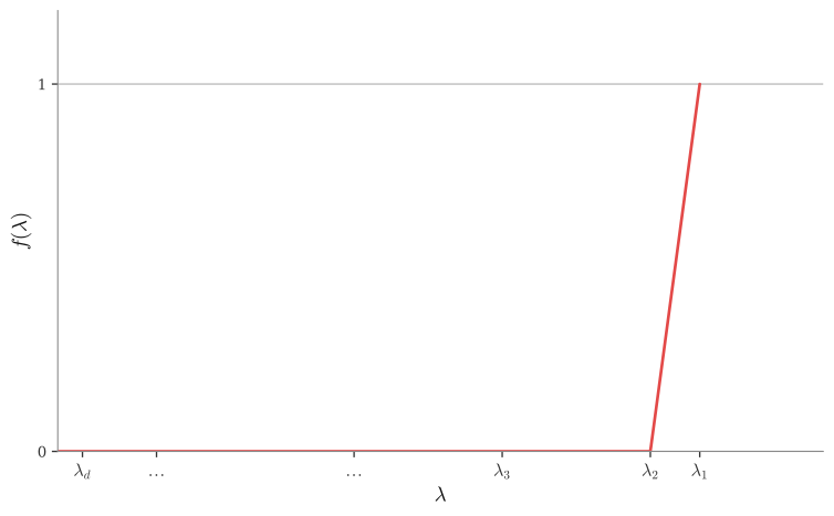
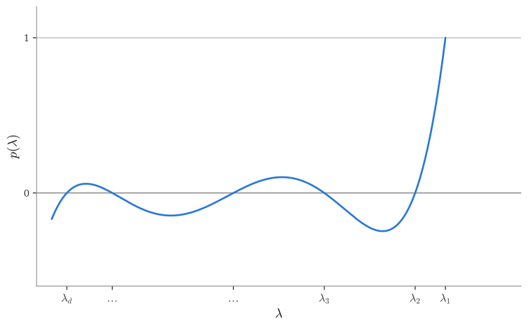
Unfortunately, we are restricted to degree-$m$ polynomials. If we try to approximate Graph 2, we might have uncovered roots where we’re far from 0, as seen in the local extrema of the graph. Instead, the safer bet seems to be finding the best degree-$m$ polynomial approximation of Graph 1, where we try to minimise our maximum distance from $0$ on $[{\lambda }_n,{\lambda }_2]$.

▶

Functional analysis helps us confirm these exact two intuitions.

For notational convenience, we define $\mathbf{z}$ to be our normalized initial vector ${\mathbf{z}}^{(0)}$.

Definition 1. Let the spectral measure ${\mu }_{\mathbf{z}}:\mathcal{B}\to \mathbb{R}$ be defined as

$${\mu }_{\mathbf{z}}(S):={\mathbf{z}}^{\top }\left(\sum _{i\ge 2}({\mathbf{v}}_i{\mathbf{v}}_i^{\top }){\delta }_{{\lambda }_i}(S)\right)\mathbf{z}$$

where the delta function is defined ${\delta }_{{\lambda }_i}(S)=\{0\text{if}{\lambda }_i\notin S,1\text{if}{\lambda }_i\in S\}$

Note that the $i\ge 2$ is not standard. It’s a choice we make because we’re only minimizing over the range $[{\lambda }_d,{\lambda }_2]$ and not on ${\lambda }_1$

Ignoring the excessive notation I have just introduced, the idea is fairly straightforward. The spectral measure ${\mu }_{\mathbf{z}}$ is a function tied to our matrix $\mathbf{A}$ and initial vector $\mathbf{z}$. It always returns the quadratic form of the initial vector with respect to $\mathbf{A}$, but it restricts its attention to the eigenvectors of $\mathbf{A}$ which happen to be in $S$. $S$ can be any set of real numbers²⁴.

Definition 2. Let the function norm $L^2({\mu }_{\mathbf{z}})$ be defined such that

$$||f|{|}_{L^2({\mu }_{\mathbf{z}})}^2=\int f(x{)}^{2}d{\mu }_{\mathbf{z}}(x)$$

This notation is designed to be extremely general for function spaces. But, we know that our spectrum of ${\lambda }_i$‘s is discrete. So, the $d{\mu }_{\mathbf{z}}(x)$ will only assign non-zero weight at the ${\lambda }_i$‘s and we can convert this to a sum. Secondly, we know we’re only applying this to polynomials $p$, not general $f$.

$$||p|{|}_{L^2({\mu }_{\mathbf{z}})}^2=\sum _{i\ge 2}p({\lambda }_i{)}^2{\mu }_{\mathbf{z}}({\lambda }_i)$$

Hopefully this is already looking familiar. It’s helpful to observe that ${\mu }_{\mathbf{z}}({\lambda }_i)$ is passing in the singleton set $S=\{{\lambda }_i\}$ to our definiton of ${\mu }_{\mathbf{z}}$, so the ${\delta }_{{\lambda }_i}$ will collapse the sum to the single term ${{\mathbf{z}}^{\top }\mathbf{v}}_i{\mathbf{v}}_i^{\top }\mathbf{z}$. So,

$$\sum _{i\ge 2}p({\lambda }_i{)}^2{\mu }_{\mathbf{z}}({\lambda }_i)={\mathbf{z}}^{\top }\left(\sum _{i\ge 2}p({\lambda }_i{)}^2{\mathbf{v}}_i{\mathbf{v}}_i^{\top }\right)\mathbf{z}=||p(A)\mathbf{z}|{|}^2$$

where the last term is in the usual vector norm, and is exactly the quantity our Lanczos method is trying to minimize! However, as we saw from our definitions, the function measure $L^2({\mu }_{\mathbf{z}})$ will depend on the spectrum of $\mathbf{A}$; if we exactly knew the spectrum of $\mathbf{A}$ we would already be done. But since $\mathbf{A}$ can be anything, there are adversarial worst-cases.

To be more precise about the problem, the $L^2$ norm is expressive of the structure of the spectrum. If you choose to go about some minimization process of $L^2$, you’re committing to a minimization based on that structure. Then, whatever guarantee you get stops holding as soon as $\mathbf{A}$ changes because the spectrum changes. This explains why approximating Graph 2 would not work: No matter what $p$ we choose, there could exist some $\mathbf{A}$ whose $\mu$ was bad for us.

We bent over backwards setting up things in the language of functional analysis above, precisely because it unlocks standard result from functional analysis for us! In particular, for any $L^p$ norms of functions for $1\le p\le \infty$²⁵:

$$||\cdot |{|}_{L^2(\mu )}\le ||\cdot |{|}_{L^3(\mu )}\le \cdots \le ||\cdot |{|}_{L^{\infty }([0,{\lambda }_2])}$$

Note: we use $[0,{\lambda }_2]$ because we know our spectrum lies there and it makes analysis easier

The key thing to notice here is, only once we reach the limit $\infty$ do we have uniform norm over the interval $[0,{\lambda }_2]$. So,

1. There are no more adversarial worst cases. Minimizing $p$ with this measure applies over the whole range $[0,{\lambda }_2]$.
2. By the monotonicity property shown above, whatever bound we find on $||p|{|}_{L^{\infty }([0,{\lambda }_2])}$ will apply to our goal of bounding $||p|{|}_{L^2(\mu )}$

So, our new goal is to find $p$ whose absolute value is minimal on the interval $[0,{\lambda }_2]$. That is, $p$ which most closely approximates $p\equiv 0$, which explains why approximating Graph 1 is the correct choice!

Of course, the degree-$0$ approximation $p\equiv 0$ literally exists. So we restrict our domain to $\{p:p({\lambda }_1)=1\}$

---

Now we’re in a good place, with a well-defined problem. Find the best degree-$m$ polynomial $p$ such that $p({\lambda }_1)=1$ and $p$ is minimized on $[0,{\lambda }_2]$

To begin with, a good intuition for how to use our $m$ degrees is as follows. Suppose we want to minimise the maximum absolute value the function achieves on the interval to some upper bound $M$. Then, we should let our polynomial curve in that direction till it hits $M$, and use our next degree $m$ to bend it back in the opposite direction trying to keep it in the $[-M,M]$ ribbon.

degree-4 p

k =4

---

It turns out this intuition is almost perfect. Approximation theory formalizes this idea with the Equioscillation Theorem.

First, define $||p||:={\max }_{x\in [-1,1]}|p(x)|$

Theorem 3 (Equioscillation Theorem). A polynomial $p^{\ast }$ of degree $\le m$ minimizes $||p||$ constrained to $p(1+ϵ)=1$ for $ϵ>0$ if and only if there exist $m+1$ points $-1\le x_0<x_1<\cdots <x_m\le 1$ at which $p^{\ast }$ attains its maximum absolute value $||p^{\ast }||$ with alternating signs, i.e.

$$p^{\ast }(x_j)=\sigma \cdot (-1{)}^j||p^{\ast }|{|}_{[-1,1]}\text{for}j=0,1,\dots ,m$$

where $\sigma =-1$ or $1$ determines the sign of the first extremum.

▶Proof of the Equioscillation Theorem

Forward direction. Suppose $p^{\ast }$ is optimal. We will show that it must equioscillate.

Suppose, for contradiction, $p^{\ast }$ does not equioscillate. We will show that some other polynomial is better, contradicting optimality.

Order the extremal points and look at the sign sequence of $p^{\ast }$ on them. Since full alternation with $m+1$ points fails, there are at most $m$ alternating points, and therefore at most $k$ sign alternations among extremal points for some $k\le m-1$. So, we can partition $[-1,1]$ into $k+1\le m$ non-empty subintervals $I_0,\dots ,I_k$ (separated by cut points $t_1<\cdots <t_k$ chosen in the gaps between the last extremal point of one sign and the first of the next) so that within each $I_i$ all extremal points share one sign, and these signs alternate from block to block.

Using the cut points $t_1,\dots ,t_k$ of this partition, we will construct a correction polynomial. Define

$$q(x)={\sigma }_q\prod _{i=1}^k(t_i-x)$$

where again, ${\sigma }_q=-1$ or $1$ just allows us to flip sign, so $q(x)$ is a polynomial of degree $k\le m-1$. Since $q$ is constructed to have roots at exactly the cut points of the intervals $I_i$, it has constant alternating sign on each block $I_i$, just like $p(x)$. Choose ${\sigma }_q$ so that $q(x)$ agrees with $p^{\ast }(x)$ on all intervals. Then, $q(x)p^{\ast }(x)>0$ everywhere on $[-1,1]$. This fact will help our analysis of the correction.

Now, we perturb $p(x)$ by some small amount $\nu$ to show an improvement. Consider the improved function

$$\tilde{p}(x)=p^{\ast }(x)-\nu \tilde{q}(x)$$

We would have just used $p^{\ast }(x)-\nu q(x)$, but we need to preserve the original constraint that $\tilde{p}(1+ϵ)=1$. So, $\tilde{q}(x)$ is just $q(x)$ modified so that $\tilde{q}(1+ϵ)=0$.

For completeness, we do this by defining $\tilde{q}(x)=q(x)-\frac{q(1+ϵ)}{r(1+ϵ)}r(x)$ where $r$ is a suitable polynomial. We can define $r=(x-(1+\frac{ϵ}{2}))q(x)$. Really $r$ can be any root between $1$ and $1+ϵ$ times $q(x)$, just so that $r$ has opposite sign structure to $q$ on $[-1,1]$ but then the same sign at $1+ϵ$, so $q(1+ϵ)/r(1+ϵ)$ is positive. Then, looking back at the definition of $\tilde{q}(x)$, we know that $-\frac{q(1+ϵ)}{r(1+ϵ)}r(x)$ shares sign with $q(x)$, so $\tilde{q}$ retains its sign from $q$ on $[-1,1]$ and $\tilde{q}(1+ϵ)=0$. We added a degree to $q$, but we were at $k\le m-1$ so it’s safe now to go to $k\le m$.

So now, $\tilde{p}(x)$ is valid candidate, and we show that it’s an improvement. Consider ${\tilde{p}}^2$.

$$\tilde{p}(x{)}^2=p^{\ast }(x{)}^2-2\nu \tilde{q}(x)p^{\ast }(x)+{\nu }^2\tilde{q}(x{)}^2=p^{\ast }(x{)}^2-2\nu (\tilde{q}(x)p^{\ast }(x)-\nu \tilde{q}(x{)}^2)$$

Remember from above that $\tilde{q}(x)p^{\ast }(x)>0$. So, for small enough $\nu$, we get $(\tilde{q}(x)p^{\ast }(x)-\nu \tilde{q}(x{)}^2)>0$. Therefore, on the whole interval, including extreme points, $\tilde{p}(x{)}^2=p^{\ast }(x{)}^2-2\nu (\text{a small positive quantity})$. So their absolute value has shrunk at the extreme points and $p^{\ast }$ was not optimal, thus a contradiction.

So, if $p^{\ast }$ is optimal, it must equioscillate.

---

Backward direction. Suppose $p^{\ast }$ equioscillates at $m+1$ points $x_0<\cdots <x_m$ with alternating signs and norm $M$. We will show that it must be optimal.

Let $p$ be any other feasible polynomial with $||p||\le M$. Consider the difference

$$d=p^{\ast }-p,\text{deg}d\le m,d(1+ϵ)=1-1=0$$

At each $x_j$, $p^{\ast }(x_j)=\pm M$ with alternating sign, and $|p(x_j)|\le M$, so,

$$d(x_j)=p^{\ast }(x_j)-p(x_j)$$

has the same sign as $p^{\ast }(x_j)$ or is zero. So $d$ takes values that alternate in sign (weakly) across the $m+1$ points $x_0,\dots ,x_m$.

A weak sign alternation across $m+1$ points forces $d$ to have at least $m$ zeros in $[-1,1]$ (counting a sign change or a shared zero in each of the $m$ consecutive gaps; strict alternation gives genuine roots, and the degenerate cases where $d(x_j)=0$ only add roots). Together with the constraint zero $d(1+ϵ)=0$ at a point outside $[-1,1]$, distinct from those $m$ zeros, so $d$ has at least $m+1$ zeros. But $d$ is a difference of two polynomials of degree at most $m$ and so can have at most $m$ roots. Therefore,

$$d\equiv 0,⟹p^{\ast }\equiv p$$

So, not only does equioscillation guarantee $p^{\ast }$ is optimal, it proves that the solution is unique.

---

We have proved the Equioscillation Theorem for $[-1,1]$ and a fixed point $1+ϵ$. It is clear to see that the polynomial can be affinely transformed to any interval, and any fixed point and still hold the same guarantees. We can use an affine change of variables to make the same claim for $p(\lambda )$ on $[0,{\lambda }_2]$ constrained to $p({\lambda }_1)=1$.

So, we know we need a polynomial that equioscillates $m$ times. The natural next question is how do we define this function.

If I have seen further, it is by standing on the shoulders of giants,
— Isaac Newton

We turn to the best, most classic equioscillator we know: the cosine function. In fact, the cosine function was screaming the answer at us all along. If we go back to the Taylor series definition of cosine we get

$$\cos (x)=1-\frac{x^2}{2!}+\frac{x^4}{4!}-\frac{x^6}{6!}\cdots =\sum _{i=0}^{\infty }\frac{(-1{)}^n}{(2n)!}{x}^{2n}$$

It literally uses each successive degree of its polynomial with alternate sign $\pm$ to stay perfectly inside $\pm 1$, and converges to the cosine at $\infty$. We, however, are restricted to finite degrees. So what cosine-like polynomial do we choose?

Well, we haven’t extracted all our mileage out of the Equioscillation Theorem yet. It gave us two pieces of information.

1. Value information: At the alternation points $-1\le x_0<x_1<\cdots <x_m=1$, $p(x_j)=\pm M$
2. Derivative information: at the alternation points, $p$ is achieving its maximum or minimum, so, if it’s interior in $(-1,1)$ then $p^{\prime }(x_j)=0$. Crucially, we know how many such points there are but not where they are. Any successful argument must somehow not need their locations.

Observe that $p^{\prime }(x)$ has degree $m-1$, but there are $m+1$ extremal points which were candidates to form the roots of $p^{\prime }(x)$. So two of the extremal points were not interior, forcing them to be on the boundaries $p(-1)=\pm M$ and $p(1)=\pm M$; we can multiply those in ourselves. And, squaring the $p^{\prime }$ part, we get $(M^2-x^2)p^{\prime }(x{)}^2$ with $2(m-1)+2=2m$ roots exactly at the equioscillation points.

Now consider $M^2-p(x{)}^2$. This will have roots exactly where $p(x)=\pm M$ and because $p$ has at exactly $m+1$ distinct points where it hits $\pm M$, $M^2-p(x{)}^2$ will have $m+1$ roots. The interior points will have multiplicity 2 and the boundaries will have multiplicity 1. So $M^2-p(x{)}^2$ will have $2(m-1)+2=2m$ roots exactly at the equioscillation points.

Lastly, it is well-established that polynomials are uniquely determined by their roots, upto a constant multiplier. We have shown that both these polynomials have equal degree and have roots exactly at the equioscillation points. So they must be equal up to a constant $C$, giving us the ODE:

$$(M^2-x^2)p^{\prime }(x{)}^2=C(M^2-p(x{)}^2)$$

Finally, solving this differential equation using standard techniques (out of scope here) reveals that the solution must be:

$$p(x)=\pm M\cos \left(m\arccos \frac{x}{M}\right)$$

It can be easily verified by using the useful substitution of $x=\cos \theta$ on $[-1,1]$ or $x=\cosh \theta$ outside $[-1,1]$ that this exactly matches the Chebyshev polynomials of the first kind²⁶

Notably, on the $[-1,1]$ range we get

$$T_n(\cos \theta )=\cos (n\theta )$$

exactly as we were trying to do before! And this confirms that our equioscillation is from $[-1,1]$

So, we have finally proved constructively that the Chebyshev polynomials are the optimal choice for this setting. Specifcally, arbitrarily letting $M$ equal $1$ they are defined by the recurrence

$$T_{n+1}(x)=2x{T}_n(x)-T_{n-1}(x),T_0(x)=1,T_1(x)=x$$

and it achieves equioscillation at magnitude $1$.

---

As a last step, in our original formulation, we wanted to construct using the inverse question: “If I have spectral gap $\gamma$, what degree $m$ do I need to suppress down to $ϵ$?”

Let $\ell (x)=\frac{2x}{{\lambda }_2}-1$ be the affine transform and take the scaled Chebyshev filter

$$p(x)=\frac{T_m(\ell (x))}{T_m(\ell ({\lambda }_1))}$$

note that the denominator is a constant.

By construction $p({\lambda }_1)=1$ and since $T_m(\ell ([0,{\lambda }_2]))=T_m([-1,1])$ and we know on $T_m([-1,1])\mapsto [-1,1]$. So,

$$\underset{[0,{\lambda }_2]}{\max }|p|=\frac{1}{T_m(\ell ({\lambda }_1))}$$

Everything now hinges on how large $T_m(\ell ({\lambda }_1))$ is. By rearranging the definition, observe that $\ell ({\lambda }_1)=\frac{1+\gamma }{1-\gamma }>1$, using our spectral gap parameter $\gamma$.

We know for $u>1$ that

$$T_m(u)=\cosh (m\mathrm{arccosh}u)$$

and we know by definitions of cosh and arccosh that

$$\cosh (m\mathrm{arccosh}u)=\frac{1}{2}\left({\rho }^m+{\rho }^{-m}\right)\text{where}\rho =u+\sqrt{u^2-1}$$

For $u=\frac{1+\gamma }{1-\gamma }$, we get $\rho =\frac{1+\sqrt{\gamma }}{1-\sqrt{\gamma }}$. And using the Taylor series of $\ln$, we get that $\ln (\frac{1+\sqrt{\gamma }}{1-\sqrt{\gamma }})\ge 2\sqrt{\gamma }$. Or equivalently, $\frac{1+\sqrt{\gamma }}{1-\sqrt{\gamma }}\ge e^{2\sqrt{\gamma }}$. Putting this together we get,

$$T_m(u)=\frac{1}{2}({\rho }^m+{\rho }^{-m})\ge \frac{1}{2}{\rho }^m\ge \frac{1}{2}{e}^{2m\sqrt{\gamma }}$$

So, to achieve $\frac{1}{T_m(u)}=\frac{1}{2}{e}^{-2\sqrt{\gamma }}\le ϵ$, we need

$$m=O(\frac{\log (1/ϵ)}{\sqrt{\gamma }})$$

Lastly, notice that we have $d-2$ more ${\lambda }_i$‘s, and in the worst case, they might all be aribtrarily close to ${\lambda }_2$. Therefore, if we wanted to suppress the sum of all of them to be less than $ϵ$, we would need a new ${ϵ}^{\prime }$ on the order $O(ϵ/d)$. Plugging this in, we finally match our bound from Claim 2

$$m=O(\frac{\log (d/ϵ)}{\sqrt{\gamma }})$$

and we are done.

---

overlay x^m?

Solve for mChoose m

degree-3 Chebyshev filter p

minimum m = 3·max |p| ≈ 0.0101·p(λ₁)/max |p| ≈ 99

γ

p(λ₁)

ε

---

Recap

To sum up, the steps we took to improve the Lanczos Method’s improvement over the Power Method were:

1. We proved that the Lanczos Method’s response $\mathbf{y}$ gets arbitrarily close to whatever optimal response there may have been ${\mathbf{y}}^{\ast }$ in the Krylov Subspace
2. We claimed that there existed at least some vector in the Krylov Subspace that was much better than the Power Method’s response (and thus the Lanczos method gets arbitrarily close to that improvement).
3. We showed that all vectors in the Krylov subspace were generated by a polynomial function.
4. We set up a relevant minimax problem over the space of constrained polynomials where we wanted $p({\lambda }_1)$ to be fixed to $1$ and then the remaining ${\lambda }_i$‘s shurnk as small as possible.
5. We proved that regardless of which specific polynomial was best, it must equioscillate
6. Finally, we proved that if it equioscillated, then it must be the Chebyshev polynomial (affinely transformed)

Footnotes

1. Of course, applied maths, as the name suggests, does not fall under this category of criticism. But then again, if your maths isn’t primarily proof-based… is it really maths? ↩

2. (1) Educator in the subject. (2) Academic who writes for other academics in the subject ↩

3. In fact I had to word my previous comment kind of carefully, because it seems maths majors are increasingly hired for this kind of thinking and exposure to rigor. ↩

4. This statement should actually be quite funny after you read the whole article. ↩

5. For any CS or maths major who has the chance to study at the Claremont Colleges, these were MATH126 and MATH138 respectively. 10/10, would recommend. ↩

6. To paraphrase Dr. Doofenshmirtz, “If I had a nickel for every time the exact same concept came up in two different college classes on the same day, I’d have three nickels—which isn’t a lot, but it’s weird that it happened thrice, right?”.
   For reference, the other two (and a half?) times are: (1) Markov’s inequality in MATH157 Probability and MATH137 Measure Theory; (2) Bellman-Ford in CS140 Algorithms and MATH187 Operations Research as LP-duality; (2.5?) Lagrange Multipliers again in MATH187, and in Multivariable Calc which I was TAing. ↩

7. Or here, functional analysis. I fear I may have ruined the joke by explaining it. ↩

8. For a matrix $\mathbf{X}$, the Gram matrix is ${\mathbf{X}}^{\top }\mathbf{X}$. It turns out that this matrix is guaranteed to be square and symmetric, which is sufficient for it to have a complete orthonormal eigendecomposition (a thing we love!) ↩

9. which is practically all problems today ↩

10. It also turns out that computing just the top singular value is enough, because we can “slice” (or more accurately “project”) off that top singular value, and then repeat the method to get the new top (formerly second-largest) singular value, and continue $k$ times. ↩

11. $[d]$ here is notation for the integer indexing set $\{1,2,\dots ,d\}$. ↩

12. I try to gloss over some of the intricacies here, so I recommend reading the notes for a more thorough treatment. ↩

13. Interestingly, this initial vector is the only place where randomness enters our algorithm. The Gaussian choice $\mathcal{N}(0,{\mathbf{I}}_d)$ is convenient for analysis, but really any random choice works because it makes adversarial worst cases extremely unlikely. ↩

14. While yes, the value of $S$ does depend on the matrix and the initial vector, the important thing is it does not change the direction of vectors at any stage, so we preserve the thing we actually care about—the direction pf the largest right-singular vector. ↩

15. That is, changing to a different orthonormal basis, like we did here ${\mathbf{v}}_1,\dots ,{\mathbf{v}}_{\mathbf{d}}$, does nothing to the distribution of the coordinates. ↩

16. with high probability. This convention in randomized algorithms says that a condition becomes vanishingly improbable. Here, for even a modest size of $d$ like $20$, we get a $>99.99\%$ guarantee. ↩

17. the choice of $m$ here may seem arbitrary, but the “convenience” here is slotting it nicely into our analysis later ↩

18. Intuitively, we can choose a threshold $ϵ$ to be as small as we need, and be guaranteed that either ${\mathbf{z}}^{(m)}$ is $ϵ$-close to ${\mathbf{v}}_1$, or it’s $ϵ$-close to $-{\mathbf{z}}^{(m)}$. Notice that they’re both good enough because we can take our singular value to be $\pm {\sigma }_1$. ↩

19. The intuitive way to see this is to imagine you have a budget of 1 because we’re restricted to unit vectors, and you have to distribute that budget over the $d$ eigenvectors to maximize the total size. You know by definition that eigenvector ${\mathbf{v}}_1$ gets the biggest multiplier ${\lambda }_1$, so the maximizing choice to put all your budget on ${\mathbf{v}}_1$ and none anywhere else. ↩

20. The proof follows almost identically for $⟨-{\mathbf{v}}_1,{\mathbf{y}}^{\ast }⟩\ge 1-2\delta /\gamma$ ↩

21. Because that’s the real fun part of this blog post! ↩

22. For reference, with $\gamma =0.0001$, the power method needs on the order of $10000$ passes over the data per factor of $\log (d/ϵ)$, while Lanczos needs on the order of $100$. ↩

23. If you’ve taken a course in Real Analysis, this may have pricked up your ears, because the Stone-Weierstrass Theorem tells us we can approximate any function arbitrarily well with polynomials. So, this may seem like a very natural/intuitive position to be in. ↩

24. Technically, we’ve defined ${\mu }_{\mathbf{z}}$ as taking only Borel sets, but distinction is not relevant; those cover all non-pathological sets we might actually need to use. ↩

25. Technically, this comes from Hölder’s inequality and relies on the spectral measure $\mu$ being no more than $1$ on the space, but that is a given from our normalization of $\mathbf{z}$ ↩

26. Chebyshev Polynomials ↩